How Much is Your Concert Ticket Really Worth?

If you are a live music aficionado, you probably have that one friend who bragged about how she made a thousand dollars flipping Coachella tickets, or tickets for some other event that are expensive and difficult to obtain. You’ve probably struggled to snag affordable tickets off of Facebook for that one event you were dying to go to, then also bought tickets off of someone for so cheap you were afraid it was a scam.
I’ve had all of these experiences, and often struggled to understand the logic of how people price tickets on the secondary market. Is there a method to all of this madness? Thankfully, there is data science to help us make sense of the market and pricings. To answer this question, I harnessed the power of Python and machine learning packages like Pandas and SciKit Learn to uncover the most important factors in the secondhand market pricings of concert tickets in the United States.
Data Gathering
For this project, I gathered event information and face value prices for live music events across the US via the Ticketmaster API. I then downloaded resale price data from the Stubhub and SeatGeek APIs, and created a list of unique artists which was then used to get artist popularity and follower data from Spotify.
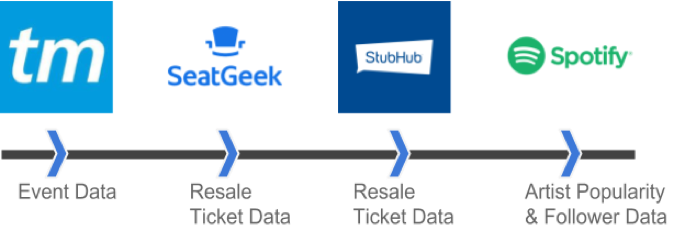 Figure 1. Data collection process, from initial event data and face value prices, to resale prices and information, and artist data from Spotify
Event listings were matched on date, venue location, and fuzzy-matched on venue name using the SeatGeek FuzzWuzzy package. Although I had gathered data for about 10,000 events, I was only able to match venue names for about 40% of them, meaning a lot of data was lost in the process. For the sake of consistency, all data was gathered on December 7, 2017.
Data Cleaning, Wrangling, and Processing
A quick look at the data revealed duplicate entries and tickets for event parking passes. There were also a handful of events with artists that aren’t on Spotify, or incorrectly entered. These values were imputed using the popularity and follower medians of each genre. Seventy-four events were also missing Ticketmaster sale start dates, which were imputed using the average number of days that all shows had been on sale.
A number of new features were created such as the number of days until a show, day of the week, length of presale, number of artists per event, average minimum and maximum resale prices (based on data from SeatGeek and Stubhub), resale ticket source, minimum and maximum markup, and the average number of resale tickets listed on a platform. Events in categories with few samples were dropped, as well as all events taking place in May 2018 or later (6+ months in the future from when the data was gathered).
Summary Statistics
After plotting CDFs and histograms, I discovered that ticket prices roughly followed a logarithmic distribution. The ticket prices data contained lots of noise, and after investigating outliers using the Tukey method, I decided to focus my analysis on comparing Ticketmaster minimum prices to resale minimums.
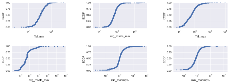 Figure 2. CDF plots of Ticketmaster ticket prices (As TM), resale prices, and markups as a percent of the Ticketmaster prices, with log-transformed Y scales.
Data Exploration
I explored the dataset with scatterplots, count plots, and statistical tests. Interestingly, New York had by far the highest markups, while California, despite being home to events like Coachella, Stagecoach, and Outside Lands, was close to the mean.
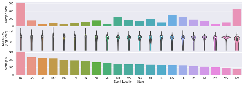 Figure 3. Ticket markups by state.
Markups don’t appear correlated to cost of living or event size. There could be a correlation between popular subgenres and markup by state, and promoter and markup by state.Markups in southern states like Louisiana and Georgia were also surprisingly high, which seems to connected to the fact that folk, country, and soul events had high markups.
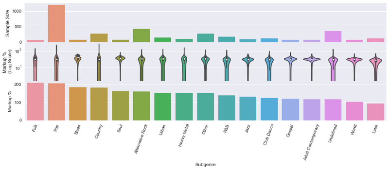 Figure 4. Ticket markups by event subgenre.
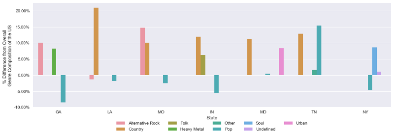 Figure 5. Top 3 subgenres by state, proportional to the overall national average.
States with high overall ticket markups also had greater concentrations of events in genres with high markups, like Country, Folk, and Soul.Events from small tour promoters or venue-promoted events also had higher markups than events by major companies like Live Nation. This suggests that smaller events might cater to more niche and dedicated audiences, or that smaller promoters simply don’t have the resources to accurately price events.
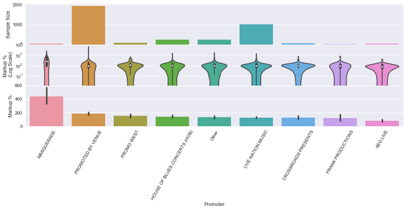 Figue 6. Ticket Markups by Promoter. Large promoter companies like Live Nation and AEG Live had much lower markups compared to events by Masquerade, and venue-promoted events.Continuous features were also analyzed by computing R2 values. I included Spearman R2 values since the pricing data is logarithmic, to determine whether a positive or negative direction correlation existed, regardless of how linear it might be.
Table 1. Pearson R and Spearman R correlations for continuous features and markup. The Ticketmaster minimum price, number of days until a show, and the number of artists per event do not have statistically significant correlations at the .05 alpha level.The correlations suggest that the higher number of tickets that are available on the resale market, the lower the markup, which intuitively makes sense from a supply and demand standpoint. In addition, having a lot of artists perform at a single event does not make a ticket more expensive on the secondary market. I found it quite interesting that several features such as the number of Spotify followers and days until a show were statistically significant but had differing sign values for Spearman and Pearson R2 values. Rather than analyze each feature and its correlation independently, we can use machine learning in the next section for a more comprehensive multivariate analysis.
Machine Learning
After collecting the data, cleaning it, and poking around to find interesting insights, it’s time for machine learning. I preprocessed the data by one-hot-encoding categorical features, standardizing independent variables to have a mean of zero and standard deviation of 1, and splitting the data into training and test sets. I used 5-fold cross validation on the training set to evaluate each machine learning algorithm I tested. I also created a second array of the dependent variable (ticket markups) and log-transformed the data, as it seemed to follow a logarithmic distribution.
I evaluated a variety of linear regression algorithms using both the log-transformed and non-transformed dependent variable array. After analyzing over a dozen linear regression methods, I concluded that the LASSO linear regression algorithm, using log-transformed Y, produced the most ideal results, as it narrowed the dataset from 74 features to 14, and had a mean absolute error of 0.6741 (on the log scale) on the training set, or 1.96% of a ticket’s markup percentage. The same algorithm produced similar results on the test set, suggesting it generalized well and was not overfitting.
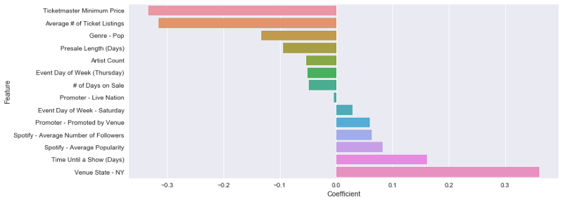 Figure 7. Coefficients of LASSO-Selected Features, on a standardized scale
The 14 features chosen by the LASSO algorithm and their coefficients provide an easy-to-understand explanation of what factors drive concert ticket markups on the secondary market. Events in New York, that are far in the future, and featured artists that are popular on Spotify demanded the highest markups, while events with high face value prices, lots of tickets on resale platforms, and pop music events drove markups down. Its important to note that all coefficients are on a standardized scale, meaning that they can be interpreted relative to one another, but not literally. In addition, although steps were taken to avoid collinearity, (such as setting drop_first to True in one hot encoding) there is always a risk of collinearity affecting the interpretability of regression coefficients.
I could have called it quits then, but decided to attempt machine learning from a different approach, by placing ticket markups into equally-sized buckets and turning the problem from one of regression to classification. I experimented with logistic regression, random forest, ada boosting, and gradient boosting algorithms, ensembling them into a voting classifier, and even building a simple neural net using Keras. All of the algorithms underwent hyperparameter tuning via GridSearchCV.
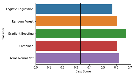 Figure 8. Accuracy scores of various classification methods after hyperparameter tuning on the test set. “Combined” is a voting classifier comprised of random forest and gradient boosting.
Although the results weren’t awful, none of the algorithms were comparable to the accuracy and interpretability of LASSO.
Conclusions
As the average ticket markup was 158%, you’re almost always best off buying tickets directly from the event promoter (Especially if you live in New York). A 158% ROI is also pretty great for anyone looking to flip tickets for extra cash, although its important to note that this project only looked at the prices of tickets that were listed on Stubhub and SeatGeek, with no way to tell how many tickets were actually sold. Still, I’d personally rather invest in concert tickets that I could enjoy if I can’t sell, rather than the latest ICO or cryptocurrency trend :)
Final Thoughts
This exercise taught me a great many things. Here a few of the major takeaways:
- Gathering your own data can be difficult especially when APIs are involved! A lot of data science advice is focused on topics like feature engineering and fine-tuning machine learning algorithms. However, one of the most challenging aspects of this project was, once finalizing my question, figuring out how to gather and stich together all the data needed. I spent much more time trying to navigate APIs then I’d care to admit, and I plan on following-up this post with a guide on the ins and outs of connecting to publically available APIs for data gathering.
-
Don’t underestimate the power of linear regression! After experimenting with neural nets and gradient boosting, I went back to linear regression as the algorithm of choice for its accurate and clearly interpretable results. For any data science problem, it’s important to understand the resources that are available to you, and who the client is. Its possible that with an additional 10,000 data points a neural net would have been worth my while, but for this project, with limited data available, and the desire to be able to explain to anyone what factors are most important in the secondary ticket market, linear regression proved to be the best.
- Have fun!
Data science is used to by big companies and startups to improve sales and cut costs but can also be used by people to answer questions that are important to them. This project has several potential business applications, but is also personally relevant to me and many others who love live music and festivals.
 ducbeo200vp 2017, “Hardwell at Ultra Music Festival Miami” — Wikimedia Commons
For a more in depth explanation of this project and its code, checkout my Python notebooks and explanations on GitHub, available here.